45 how to display data labels above the columns in excel

How to add data labels from different column in an Excel chart? Reuse Anything: Add the most used or complex formulas, charts and anything else to your favorites, and quickly reuse them in the future. More than 20 text features: Extract Number from Text String; Extract or Remove Part of Texts; Convert Numbers and Currencies to English Words. Merge Tools: Multiple Workbooks and Sheets into One; Merge Multiple Cells/Rows/Columns … chandoo.org › wp › change-data-labels-in-chartsHow to Change Excel Chart Data Labels to Custom Values? May 05, 2010 · Now, click on any data label. This will select “all” data labels. Now click once again. At this point excel will select only one data label. Go to Formula bar, press = and point to the cell where the data label for that chart data point is defined. Repeat the process for all other data labels, one after another. See the screencast.

› charts › dynamic-chart-dataCreate Dynamic Chart Data Labels with Slicers - Excel Campus Feb 10, 2016 · Step 3: Use the TEXT Function to Format the Labels. Typically a chart will display data labels based on the underlying source data for the chart. In Excel 2013 a new feature called “Value from Cells” was introduced. This feature allows us to specify the a range that we want to use for the labels.

How to display data labels above the columns in excel

How to group rows and columns in Excel | Excelchat When working with spreadsheets, a time comes when we have to group data t ogether. We can group columns based on various criteria, such as the heading or even contents of the columns. Usually, when we group adjacent cells, the group function will simply condense them into one group.. Below is a procedure on how to group columns;. Step 1: Prepare the spreadsheet with … › custom-data-labels-in-xImprove your X Y Scatter Chart with custom data labels May 06, 2021 · Thank you for your Excel 2010 workaround for custom data labels in XY scatter charts. It basically works for me until I insert a new row in the worksheet associated with the chart. Doing so breaks the absolute references to data labels after the inserted row and Excel won't let me change the data labels to relative references. helpx.adobe.com › indesign › usingMerge data to create form letters, envelopes, or mailing ... Jan 06, 2022 · The merged document maintains a connection to the data source, so if records in the data source are modified, you can update the merged document contents by choosing Update Content In Data Fields. This option is especially helpful if you change the layout in the merged document and then need to add new data from the data source.

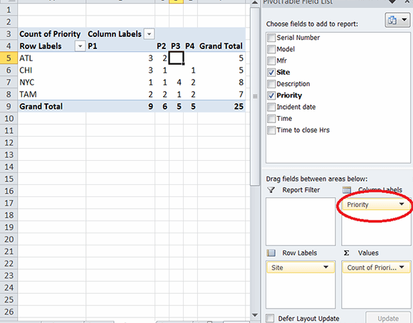
How to display data labels above the columns in excel. Excel for Commerce | Analyze large data sets in Excel 7.5.2015 · Now that you have these calculated columns, you can use filters as you did above to find the top names in each year. Select Columns A:F, and in the HOME tab, under Sort & Filter, choose Filter. Now click the filter icon in cell F1 and select only the names of rank one (i.e. the #1 names of each sex of each year). › display-missingDisplay Missing Dates in Excel PivotTables • My Online ... Mar 25, 2014 · Note: Apply 'Wrap Text' format to column B of your Table if you want to see your date text string formatted as per the image above, i.e. with the date number above the letter for the day. However, this is not necessary for the PivotChart since it wraps the text because we have used the CHAR(10) character in the text string. Display Missing Dates in Excel PivotTables - My Online Training … 25.3.2014 · Q: How do you get the PivotTable to show the missing dates in your data? A: Not as easily as it should be, but here are a couple of workarounds you can use. Option 1: If you don’t care how Excel formats your dates. The limitation of this option, as you will see, is that when Excel groups days in a PivotTable it shows the date formatted as “d-mmm” and you cannot … › excel_pivot_tables › excelExcel Pivot Tables - Areas - tutorialspoint.com Your PivotTable appears with one column containing the Row Labels – Salesperson and Month and a last row as Grand Total, as given below. COLUMNS. You can drag fields to the COLUMNS area. The fields that are put in COLUMNS area appear as columns in the PivotTable, with the Column Labels being the values of the selected fields.

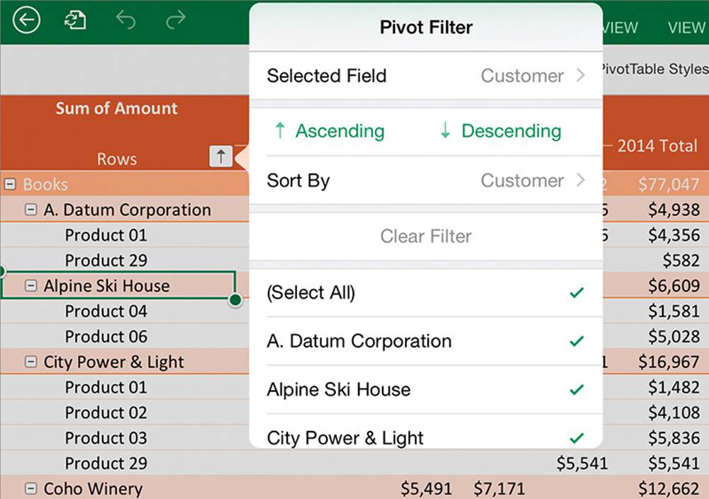
Filter data in a PivotTable You can repeat this step to create more than one report filter. Report filters are displayed above the PivotTable for easy access. To change the order of the fields, in the Filters area, you can either drag the fields to the position that you want, or double-click on a field and select Move Up or Move Down.The order of the report filters will be reflected accordingly in the PivotTable. How to Change Excel Chart Data Labels to Custom Values? 5.5.2010 · When you "add data labels" to a chart series, excel can show either "category" , ... but in my case the labels were numeric values so I just changed to a stacked bar chart and added a clear stack above the data with the values plotted as data. Reply. Ankit says: June 6, ... It will display labels 1, 4 , 6 , 7, 9 , 10, 15, ... How to group (two-level) axis labels in a chart in Excel? The Pivot Chart tool is so powerful that it can help you to create a chart with one kind of labels grouped by another kind of labels in a two-lever axis easily in Excel. You can do as follows: 1. Create a Pivot Chart with selecting the source data, and: (1) In Excel 2007 and 2010, clicking the PivotTable > PivotChart in the Tables group on the ... Excel Pivot Tables - Areas - tutorialspoint.com COLUMNS. FILTERS. ∑ VALUES (Read as Summarizing Values). The message - Drag fields between areas below appears above the areas. With PivotTable Areas, you can choose −. What fields to display as rows (ROWS area). What fields to display as columns (COLUMNS area). How to summarize your data (∑ VALUES area). Filters for any of the fields ...

Create Dynamic Chart Data Labels with Slicers - Excel Campus 10.2.2016 · Typically a chart will display data labels based on the underlying source data for the chart. In Excel 2013 a new feature called “Value from Cells” was introduced. This feature allows us to specify the a range that we want to use for the labels. Since our data labels will change between a currency ($) and percentage (%) formats, we need a ... Improve your X Y Scatter Chart with custom data labels - Get … 6.5.2021 · You can manually press with left mouse button on and drag data labels as needed. You can also let excel change the position of all data labels, choose between center, left, right, above and below. Press with right mouse button on on a data label; Press with left mouse button on "Format Data Labels" Select a new label position. Back to top › documents › excelHow to add data labels from different column in an Excel chart? This method will introduce a solution to add all data labels from a different column in an Excel chart at the same time. Please do as follows: 1. Right click the data series in the chart, and select Add Data Labels > Add Data Labels from the context menu to add data labels. 2. helpx.adobe.com › indesign › usingMerge data to create form letters, envelopes, or mailing ... Jan 06, 2022 · The merged document maintains a connection to the data source, so if records in the data source are modified, you can update the merged document contents by choosing Update Content In Data Fields. This option is especially helpful if you change the layout in the merged document and then need to add new data from the data source.

November 2018

› custom-data-labels-in-xImprove your X Y Scatter Chart with custom data labels May 06, 2021 · Thank you for your Excel 2010 workaround for custom data labels in XY scatter charts. It basically works for me until I insert a new row in the worksheet associated with the chart. Doing so breaks the absolute references to data labels after the inserted row and Excel won't let me change the data labels to relative references.